import os
import time
import httpx
import pandas as pd
import matplotlib.pyplot as plt
from dotenv import load_dotenv
load_dotenv()
BASE_URL = "https://api.openalex.org"
api = httpx.Client(
base_url=BASE_URL,
params={
"mailto": os.environ.get("OPENALEX_MAILTO", ""),
"api_key": os.environ["OPENALEX_API_KEY"],
},
timeout=30,
)
FIELDS = {
"Physics and Astronomy": "fields/31",
"Agricultural and Biological Sciences": "fields/11",
"Biochemistry, Genetics and Molecular Biology": "fields/13",
"Economics, Econometrics and Finance": "fields/20",
}
def _get(path: str, **kwargs) -> dict:
"""GET with automatic retry on 429 and connection errors."""
for attempt in range(5):
try:
r = api.get(path, **kwargs)
except httpx.ReadError:
time.sleep(2 ** attempt)
continue
if r.status_code == 429:
time.sleep(2 ** attempt)
continue
r.raise_for_status()
return r.json()
raise RuntimeError("Max retries exceeded")
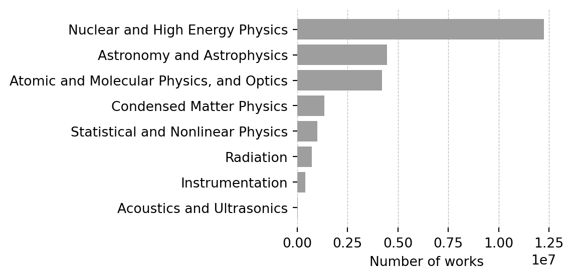
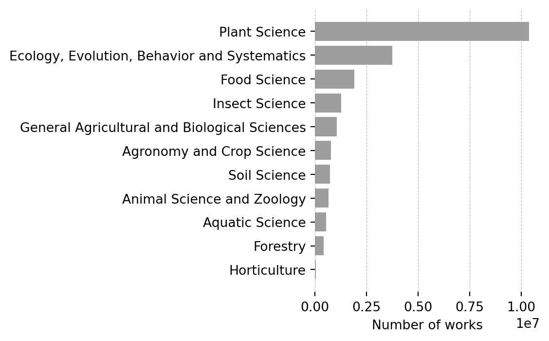
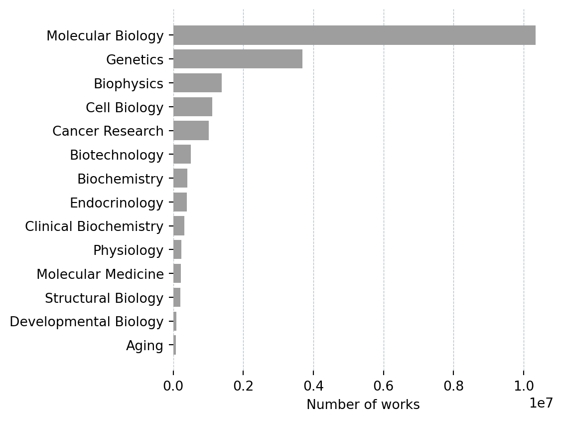
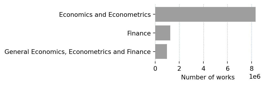
def get_subfields(field_name: str, field_id: str) -> pd.DataFrame:
data = _get("/subfields", params={
"filter": f"field.id:{field_id}",
"select": "id,display_name,works_count",
"per-page": 50,
"sort": "works_count:desc",
})
df = pd.DataFrame(data["results"])[["display_name", "works_count"]]
df.columns = ["Subfield", "Works"]
df.insert(0, "Field", field_name)
return df
BAR_HEIGHT = 0.25 # inches per bar — keeps bars the same size across charts
def plot_subfields(df: pd.DataFrame):
fig_h = max(2, len(df) * BAR_HEIGHT + 1)
fig, ax = plt.subplots(figsize=(6, fig_h))
ax.barh(df["Subfield"][::-1], df["Works"][::-1], color="#9e9e9e")
ax.set_xlabel("Number of works")
ax.grid(axis="x", color="#b0bec5", linewidth=0.5, linestyle="--")
ax.set_axisbelow(True)
for spine in ax.spines.values():
spine.set_visible(False)
plt.tight_layout()
plt.show()
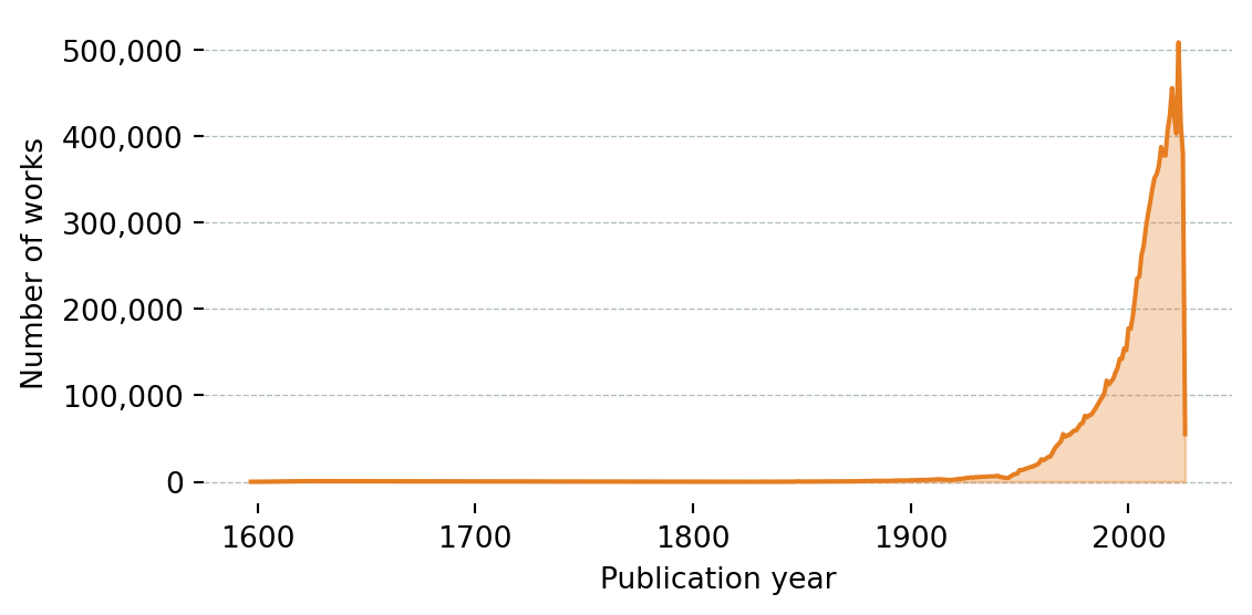
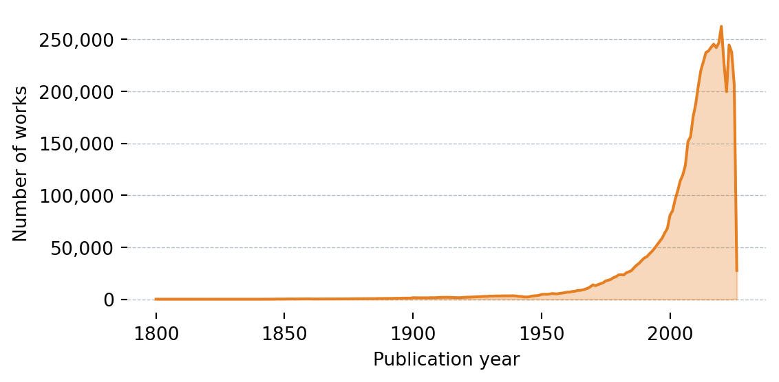
def get_works_by_year(field_name: str, field_id: str) -> pd.DataFrame:
data = _get("/works", params={
"filter": f"primary_topic.field.id:{field_id}",
"group_by": "publication_year",
})
rows = [
{"Year": int(g["key"]), "Works": g["count"]}
for g in data["group_by"]
if g["key"] != "unknown"
]
df = pd.DataFrame(rows).sort_values("Year")
df.insert(0, "Field", field_name)
return df
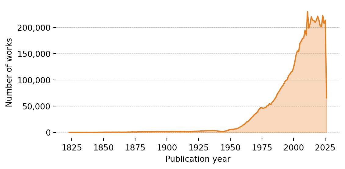
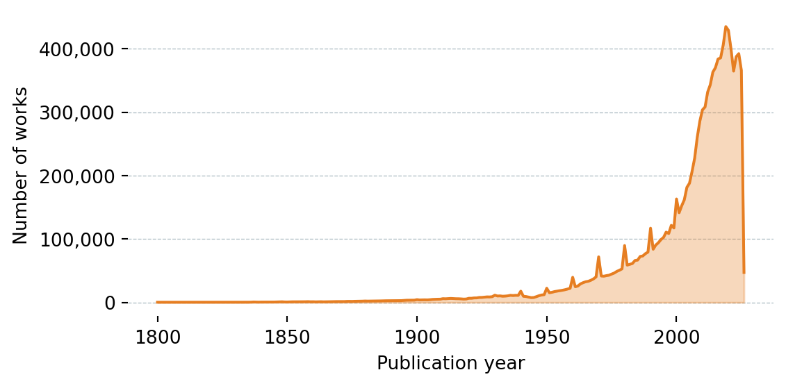
def plot_works_by_year(df: pd.DataFrame):
fig, ax = plt.subplots(figsize=(6, 3))
ax.fill_between(df["Year"], df["Works"], alpha=0.3, color="#e67e22")
ax.plot(df["Year"], df["Works"], color="#e67e22", linewidth=1.5)
ax.set_xlabel("Publication year")
ax.set_ylabel("Number of works")
ax.yaxis.set_major_formatter(plt.FuncFormatter(lambda x, _: f"{x:,.0f}"))
ax.grid(axis="y", color="#b0bec5", linewidth=0.5, linestyle="--")
ax.set_axisbelow(True)
for spine in ax.spines.values():
spine.set_visible(False)
plt.tight_layout()
plt.show()
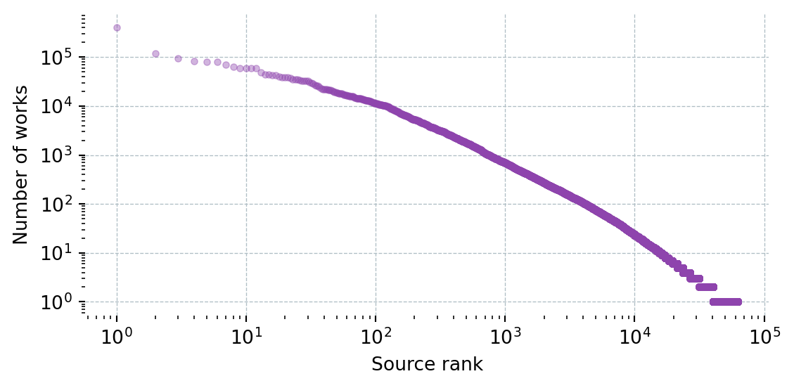
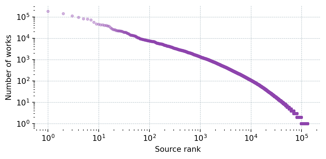
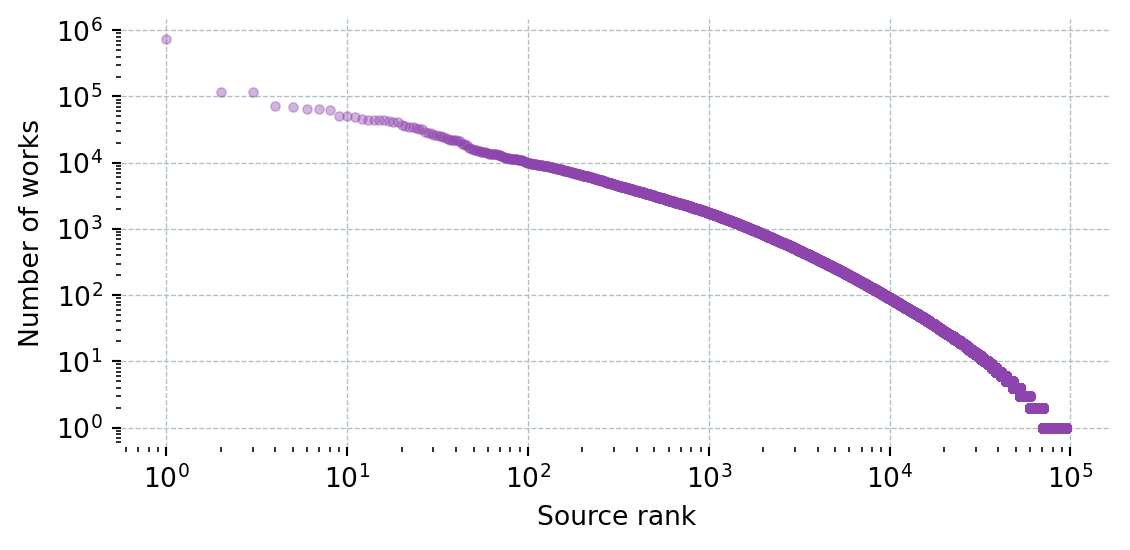
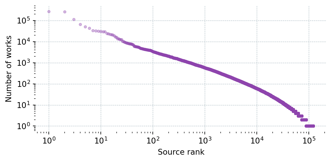
def get_works_by_source(field_name: str, field_id: str) -> pd.DataFrame:
params = {
"filter": f"primary_topic.field.id:{field_id}",
"group_by": "primary_location.source.id",
"per-page": 200,
"cursor": "*",
}
rows = []
while True:
data = _get("/works", params=params)
for g in data["group_by"]:
rows.append({"Source": g["key_display_name"], "Works": g["count"]})
cursor = data["meta"].get("next_cursor")
if not cursor or len(data["group_by"]) == 0:
break
params["cursor"] = cursor
time.sleep(0.1)
df = pd.DataFrame(rows).sort_values("Works", ascending=False).reset_index(drop=True)
df.insert(0, "Field", field_name)
return df
TOP_N_SOURCES = 20
def plot_works_by_source(df: pd.DataFrame):
top = df.head(TOP_N_SOURCES)
fig_h = max(2, len(top) * BAR_HEIGHT + 1)
fig, ax = plt.subplots(figsize=(6, fig_h))
ax.barh(top["Source"][::-1], top["Works"][::-1], color="#2980b9")
ax.set_xlabel("Number of works")
ax.xaxis.set_major_formatter(plt.FuncFormatter(lambda x, _: f"{x:,.0f}"))
ax.grid(axis="x", color="#b0bec5", linewidth=0.5, linestyle="--")
ax.set_axisbelow(True)
for spine in ax.spines.values():
spine.set_visible(False)
plt.tight_layout()
plt.show()